Use kNN model, sklearn, python and the classic iris dataset to predict flower species based on features.

About:

This case study is for phase 1 of my 100 days of machine learning code challenge.

This is a homework solution to a section in Machine Learning Classification Bootcamp in Python.

Problem Statement:

Predict Species of Iris given 4 feature measurments

  • Sepal Length (cm)
  • Sepal Width (cm)
  • Petal Length (cm)
  • Petal Width (cm)

Technology used:

Model(s):

Dataset(s):

Libraries:

Resources:

Contact:

If for any reason you would like to contact me please do so at the following:

KNN Iris Classifier

KNN used for classifier Compares to most similar data points

Import Libraries

In [1]:
import pandas as pd
import seaborn as sns
import matplotlib.pyplot as plt
%matplotlib inline

Import & Explore Data

In [2]:
iris = pd.read_csv('../datasets/iris/iris.csv')
In [3]:
iris.head()
Out[3]:
SepalLengthCm SepalWidthCm PetalLengthCm PetalWidthCm Species
0 5.1 3.5 1.4 0.2 Iris-setosa
1 4.9 3.0 1.4 0.2 Iris-setosa
2 4.7 3.2 1.3 0.2 Iris-setosa
3 4.6 3.1 1.5 0.2 Iris-setosa
4 5.0 3.6 1.4 0.2 Iris-setosa
In [4]:
iris.tail()
Out[4]:
SepalLengthCm SepalWidthCm PetalLengthCm PetalWidthCm Species
145 6.7 3.0 5.2 2.3 Iris-virginica
146 6.3 2.5 5.0 1.9 Iris-virginica
147 6.5 3.0 5.2 2.0 Iris-virginica
148 6.2 3.4 5.4 2.3 Iris-virginica
149 5.9 3.0 5.1 1.8 Iris-virginica
In [29]:
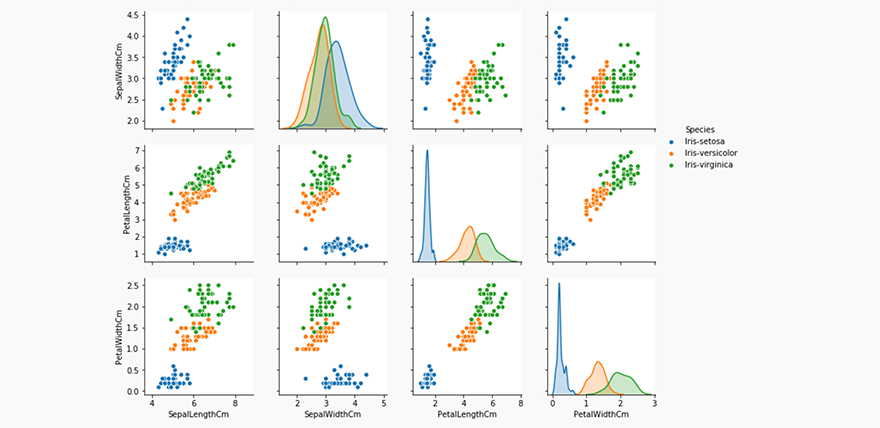
sns.pairplot(iris, hue = 'Species', vars = ['SepalLengthCm',
                                            'SepalWidthCm',
                                            'PetalLengthCm',
                                            'PetalWidthCm' ])
Out[29]:
<seaborn.axisgrid.PairGrid at 0x1a1f8c4550>
In [30]:
sns.scatterplot(x = 'SepalLengthCm',
                y = 'PetalLengthCm',
                hue = 'Species',
                data = iris)
Out[30]:
<matplotlib.axes._subplots.AxesSubplot at 0x1a1fe67f28>
In [7]:
# plot corrilations
plt.figure(figsize =(30,20))

sns.heatmap(iris.corr(), annot = True)
Out[7]:
<matplotlib.axes._subplots.AxesSubplot at 0x1199ea4e0>

Data Cleaning & Prep

In [8]:
X = iris.drop(['Species'], axis = 1)
In [9]:
X.shape
Out[9]:
(150, 4)
In [10]:
X.head()
Out[10]:
SepalLengthCm SepalWidthCm PetalLengthCm PetalWidthCm
0 5.1 3.5 1.4 0.2
1 4.9 3.0 1.4 0.2
2 4.7 3.2 1.3 0.2
3 4.6 3.1 1.5 0.2
4 5.0 3.6 1.4 0.2
In [11]:
y = iris['Species']
In [12]:
y.shape
Out[12]:
(150,)
In [13]:
y
Out[13]:
0         Iris-setosa
1         Iris-setosa
2         Iris-setosa
3         Iris-setosa
4         Iris-setosa
5         Iris-setosa
6         Iris-setosa
7         Iris-setosa
8         Iris-setosa
9         Iris-setosa
10        Iris-setosa
11        Iris-setosa
12        Iris-setosa
13        Iris-setosa
14        Iris-setosa
15        Iris-setosa
16        Iris-setosa
17        Iris-setosa
18        Iris-setosa
19        Iris-setosa
20        Iris-setosa
21        Iris-setosa
22        Iris-setosa
23        Iris-setosa
24        Iris-setosa
25        Iris-setosa
26        Iris-setosa
27        Iris-setosa
28        Iris-setosa
29        Iris-setosa
            ...      
120    Iris-virginica
121    Iris-virginica
122    Iris-virginica
123    Iris-virginica
124    Iris-virginica
125    Iris-virginica
126    Iris-virginica
127    Iris-virginica
128    Iris-virginica
129    Iris-virginica
130    Iris-virginica
131    Iris-virginica
132    Iris-virginica
133    Iris-virginica
134    Iris-virginica
135    Iris-virginica
136    Iris-virginica
137    Iris-virginica
138    Iris-virginica
139    Iris-virginica
140    Iris-virginica
141    Iris-virginica
142    Iris-virginica
143    Iris-virginica
144    Iris-virginica
145    Iris-virginica
146    Iris-virginica
147    Iris-virginica
148    Iris-virginica
149    Iris-virginica
Name: Species, Length: 150, dtype: object
In [14]:
# transform y data into digits (0,1)
from sklearn.preprocessing import LabelEncoder
labelencoder_y = LabelEncoder()
y = labelencoder_y.fit_transform(y)
In [15]:
y
Out[15]:
array([0, 0, 0, 0, 0, 0, 0, 0, 0, 0, 0, 0, 0, 0, 0, 0, 0, 0, 0, 0, 0, 0, 0,
       0, 0, 0, 0, 0, 0, 0, 0, 0, 0, 0, 0, 0, 0, 0, 0, 0, 0, 0, 0, 0, 0, 0,
       0, 0, 0, 0, 1, 1, 1, 1, 1, 1, 1, 1, 1, 1, 1, 1, 1, 1, 1, 1, 1, 1, 1,
       1, 1, 1, 1, 1, 1, 1, 1, 1, 1, 1, 1, 1, 1, 1, 1, 1, 1, 1, 1, 1, 1, 1,
       1, 1, 1, 1, 1, 1, 1, 1, 2, 2, 2, 2, 2, 2, 2, 2, 2, 2, 2, 2, 2, 2, 2,
       2, 2, 2, 2, 2, 2, 2, 2, 2, 2, 2, 2, 2, 2, 2, 2, 2, 2, 2, 2, 2, 2, 2,
       2, 2, 2, 2, 2, 2, 2, 2, 2, 2, 2, 2])
In [31]:
# Create train Test Split
from sklearn.model_selection import train_test_split
X_train, X_test, y_train, y_test = train_test_split(X,
                                                    y,
                                                    test_size=0.20,
                                                    random_state = 5,
                                                    stratify=y)
In [17]:
X_train.shape
Out[17]:
(120, 4)
In [18]:
X_test.shape
Out[18]:
(30, 4)

Train & test Model

In [19]:
from sklearn.neighbors import KNeighborsClassifier
In [32]:
classifier = KNeighborsClassifier(n_neighbors=3,
                                  metric = 'minkowski',
                                  p=2)
classifier.fit(X_train, y_train)
Out[32]:
KNeighborsClassifier(algorithm='auto', leaf_size=30, metric='minkowski',
           metric_params=None, n_jobs=1, n_neighbors=3, p=2,
           weights='uniform')
In [21]:
y_pred = classifier.predict(X_test)
In [22]:
print(y_pred)
print(y_test)
[0 0 0 2 1 2 0 0 1 1 0 0 1 2 1 2 2 2 0 1 0 1 2 1 1 0 2 2 1 1]
[0 0 0 2 1 2 0 0 1 1 0 0 1 2 1 2 2 2 0 1 0 1 2 2 1 0 2 2 1 1]
In [23]:
from sklearn.metrics import confusion_matrix, classification_report
cm = confusion_matrix(y_test, y_pred)
In [24]:
sns.heatmap(cm,annot = True)
Out[24]:
<matplotlib.axes._subplots.AxesSubplot at 0x11b1a3cc0>
In [25]:
print(classification_report(y_test, y_pred))
             precision    recall  f1-score   support

          0       1.00      1.00      1.00        10
          1       0.91      1.00      0.95        10
          2       1.00      0.90      0.95        10

avg / total       0.97      0.97      0.97        30

In [26]:
import shap
# print the JS visualization code to the notebook
shap.initjs()
In [27]:
# explain all the predictions in the test set
explainer = shap.KernelExplainer(classifier.predict, X_train)
shap_values = explainer.shap_values(X_test)
Using 120 background data samples could cause slower run times. Consider using shap.kmeans(data, K) to summarize the background as K weighted samples.
100%|██████████| 30/30 [00:00<00:00, 49.36it/s]
In [28]:
shap.summary_plot(shap_values, X_test)