Titanic Survival

About:

This project / case study is for phase 1 of my 100 days of machine learning code challenge.

This is a homework solution to a section in Machine Learning Classification Bootcamp in Python.

Problem Statement:

Predict Passenger Survival based on feature measurments of the titanic dataset.

Technology used:

Model(s):

Dataset(s):

Libraries:

Resources:

Contact:

If for any reason you would like to contact me please do so at the following:

Import Libraries

In [1]:
# import Libraries
import pandas as pd
import seaborn as sns
import matplotlib.pyplot as plt
%matplotlib inline

Import Dataset

In [2]:
#import Data into Pandas DataFrame
training_set = pd.read_csv('../datasets/titanic/Train_Titanic.csv')
In [3]:
#Verify Data imported
training_set.head(10)
# training_set.tail(10)
Out[3]:
PassengerId Survived Pclass Name Sex Age SibSp Parch Ticket Fare Cabin Embarked
0 1 0 3 Braund, Mr. Owen Harris male 22.0 1 0 A/5 21171 7.2500 NaN S
1 2 1 1 Cumings, Mrs. John Bradley (Florence Briggs Th... female 38.0 1 0 PC 17599 71.2833 C85 C
2 3 1 3 Heikkinen, Miss. Laina female 26.0 0 0 STON/O2. 3101282 7.9250 NaN S
3 4 1 1 Futrelle, Mrs. Jacques Heath (Lily May Peel) female 35.0 1 0 113803 53.1000 C123 S
4 5 0 3 Allen, Mr. William Henry male 35.0 0 0 373450 8.0500 NaN S
5 6 0 3 Moran, Mr. James male NaN 0 0 330877 8.4583 NaN Q
6 7 0 1 McCarthy, Mr. Timothy J male 54.0 0 0 17463 51.8625 E46 S
7 8 0 3 Palsson, Master. Gosta Leonard male 2.0 3 1 349909 21.0750 NaN S
8 9 1 3 Johnson, Mrs. Oscar W (Elisabeth Vilhelmina Berg) female 27.0 0 2 347742 11.1333 NaN S
9 10 1 2 Nasser, Mrs. Nicholas (Adele Achem) female 14.0 1 0 237736 30.0708 NaN C

Explore Dataset

In [4]:
survived = training_set[training_set['Survived']==1]
no_survived = training_set[training_set['Survived']==0]
In [5]:
print('Total Passengers = ', len(training_set))
print('Number of Passengers who survived = ', len(survived))
print('Number of Passengers who died = ', len(no_survived))
print('% Survived = ', 1 * len(survived)/len(training_set) * 100)
print('% Died = ', 1 * len(no_survived)/len(training_set) * 100)
Total Passengers =  891
Number of Passengers who survived =  342
Number of Passengers who died =  549
% Survived =  38.38383838383838
% Died =  61.61616161616161
In [6]:
# plot Passenger class numbers
sns.countplot(x = 'Pclass', data = training_set)
Out[6]:
<matplotlib.axes._subplots.AxesSubplot at 0x1a0d99c3c8>
In [7]:
# plot Passenger survival by class numbers
sns.countplot(x = 'Pclass', hue = 'Survived', data = training_set)
Out[7]:
<matplotlib.axes._subplots.AxesSubplot at 0x1a0d7f4438>
In [8]:
# plot Passenger siblings
sns.countplot(x = 'SibSp', data = training_set)
Out[8]:
<matplotlib.axes._subplots.AxesSubplot at 0x1a15eb57f0>
In [9]:
# plot Passenger survival with siblings
sns.countplot(x = 'SibSp', hue = 'Survived', data = training_set)
Out[9]:
<matplotlib.axes._subplots.AxesSubplot at 0x1a15fac400>
In [10]:
# plot Passengers with Parent / child
sns.countplot(x = 'Parch', data = training_set)
Out[10]:
<matplotlib.axes._subplots.AxesSubplot at 0x1a1607d2b0>
In [11]:
# plot Passenger survival with Parent / child
sns.countplot(x = 'Parch', hue = 'Survived', data = training_set)
Out[11]:
<matplotlib.axes._subplots.AxesSubplot at 0x1a161b2710>
In [12]:
# plot Passengers embarked
sns.countplot(x = 'Embarked', data = training_set)
Out[12]:
<matplotlib.axes._subplots.AxesSubplot at 0x1a162c5b70>
In [13]:
# plot Passenger survival from Embarked
sns.countplot(x = 'Embarked', hue = 'Survived', data = training_set)
Out[13]:
<matplotlib.axes._subplots.AxesSubplot at 0x1a16347c88>
In [14]:
# plot Passengers Sex
sns.countplot(x = 'Sex', data = training_set)
Out[14]:
<matplotlib.axes._subplots.AxesSubplot at 0x1a164200f0>
In [15]:
# plot Passengers Sex Survival
sns.countplot(x = 'Sex', hue = 'Survived', data = training_set)
Out[15]:
<matplotlib.axes._subplots.AxesSubplot at 0x1a161bd208>
In [16]:
# Plot survival by Age
plt.figure(figsize =  (40, 30))
sns.countplot(x = 'Age', hue = 'Survived', data = training_set)
Out[16]:
<matplotlib.axes._subplots.AxesSubplot at 0x1a165549b0>
In [17]:
training_set['Age'].hist(bins = 40)
Out[17]:
<matplotlib.axes._subplots.AxesSubplot at 0x1a169f6f60>
In [18]:
training_set['Fare'].hist(bins = 40)
Out[18]:
<matplotlib.axes._subplots.AxesSubplot at 0x1a1915dd30>

Cleaning Data

In [19]:
training_set
Out[19]:
PassengerId Survived Pclass Name Sex Age SibSp Parch Ticket Fare Cabin Embarked
0 1 0 3 Braund, Mr. Owen Harris male 22.0 1 0 A/5 21171 7.2500 NaN S
1 2 1 1 Cumings, Mrs. John Bradley (Florence Briggs Th... female 38.0 1 0 PC 17599 71.2833 C85 C
2 3 1 3 Heikkinen, Miss. Laina female 26.0 0 0 STON/O2. 3101282 7.9250 NaN S
3 4 1 1 Futrelle, Mrs. Jacques Heath (Lily May Peel) female 35.0 1 0 113803 53.1000 C123 S
4 5 0 3 Allen, Mr. William Henry male 35.0 0 0 373450 8.0500 NaN S
5 6 0 3 Moran, Mr. James male NaN 0 0 330877 8.4583 NaN Q
6 7 0 1 McCarthy, Mr. Timothy J male 54.0 0 0 17463 51.8625 E46 S
7 8 0 3 Palsson, Master. Gosta Leonard male 2.0 3 1 349909 21.0750 NaN S
8 9 1 3 Johnson, Mrs. Oscar W (Elisabeth Vilhelmina Berg) female 27.0 0 2 347742 11.1333 NaN S
9 10 1 2 Nasser, Mrs. Nicholas (Adele Achem) female 14.0 1 0 237736 30.0708 NaN C
10 11 1 3 Sandstrom, Miss. Marguerite Rut female 4.0 1 1 PP 9549 16.7000 G6 S
11 12 1 1 Bonnell, Miss. Elizabeth female 58.0 0 0 113783 26.5500 C103 S
12 13 0 3 Saundercock, Mr. William Henry male 20.0 0 0 A/5. 2151 8.0500 NaN S
13 14 0 3 Andersson, Mr. Anders Johan male 39.0 1 5 347082 31.2750 NaN S
14 15 0 3 Vestrom, Miss. Hulda Amanda Adolfina female 14.0 0 0 350406 7.8542 NaN S
15 16 1 2 Hewlett, Mrs. (Mary D Kingcome) female 55.0 0 0 248706 16.0000 NaN S
16 17 0 3 Rice, Master. Eugene male 2.0 4 1 382652 29.1250 NaN Q
17 18 1 2 Williams, Mr. Charles Eugene male NaN 0 0 244373 13.0000 NaN S
18 19 0 3 Vander Planke, Mrs. Julius (Emelia Maria Vande... female 31.0 1 0 345763 18.0000 NaN S
19 20 1 3 Masselmani, Mrs. Fatima female NaN 0 0 2649 7.2250 NaN C
20 21 0 2 Fynney, Mr. Joseph J male 35.0 0 0 239865 26.0000 NaN S
21 22 1 2 Beesley, Mr. Lawrence male 34.0 0 0 248698 13.0000 D56 S
22 23 1 3 McGowan, Miss. Anna "Annie" female 15.0 0 0 330923 8.0292 NaN Q
23 24 1 1 Sloper, Mr. William Thompson male 28.0 0 0 113788 35.5000 A6 S
24 25 0 3 Palsson, Miss. Torborg Danira female 8.0 3 1 349909 21.0750 NaN S
25 26 1 3 Asplund, Mrs. Carl Oscar (Selma Augusta Emilia... female 38.0 1 5 347077 31.3875 NaN S
26 27 0 3 Emir, Mr. Farred Chehab male NaN 0 0 2631 7.2250 NaN C
27 28 0 1 Fortune, Mr. Charles Alexander male 19.0 3 2 19950 263.0000 C23 C25 C27 S
28 29 1 3 O'Dwyer, Miss. Ellen "Nellie" female NaN 0 0 330959 7.8792 NaN Q
29 30 0 3 Todoroff, Mr. Lalio male NaN 0 0 349216 7.8958 NaN S
... ... ... ... ... ... ... ... ... ... ... ... ...
861 862 0 2 Giles, Mr. Frederick Edward male 21.0 1 0 28134 11.5000 NaN S
862 863 1 1 Swift, Mrs. Frederick Joel (Margaret Welles Ba... female 48.0 0 0 17466 25.9292 D17 S
863 864 0 3 Sage, Miss. Dorothy Edith "Dolly" female NaN 8 2 CA. 2343 69.5500 NaN S
864 865 0 2 Gill, Mr. John William male 24.0 0 0 233866 13.0000 NaN S
865 866 1 2 Bystrom, Mrs. (Karolina) female 42.0 0 0 236852 13.0000 NaN S
866 867 1 2 Duran y More, Miss. Asuncion female 27.0 1 0 SC/PARIS 2149 13.8583 NaN C
867 868 0 1 Roebling, Mr. Washington Augustus II male 31.0 0 0 PC 17590 50.4958 A24 S
868 869 0 3 van Melkebeke, Mr. Philemon male NaN 0 0 345777 9.5000 NaN S
869 870 1 3 Johnson, Master. Harold Theodor male 4.0 1 1 347742 11.1333 NaN S
870 871 0 3 Balkic, Mr. Cerin male 26.0 0 0 349248 7.8958 NaN S
871 872 1 1 Beckwith, Mrs. Richard Leonard (Sallie Monypeny) female 47.0 1 1 11751 52.5542 D35 S
872 873 0 1 Carlsson, Mr. Frans Olof male 33.0 0 0 695 5.0000 B51 B53 B55 S
873 874 0 3 Vander Cruyssen, Mr. Victor male 47.0 0 0 345765 9.0000 NaN S
874 875 1 2 Abelson, Mrs. Samuel (Hannah Wizosky) female 28.0 1 0 P/PP 3381 24.0000 NaN C
875 876 1 3 Najib, Miss. Adele Kiamie "Jane" female 15.0 0 0 2667 7.2250 NaN C
876 877 0 3 Gustafsson, Mr. Alfred Ossian male 20.0 0 0 7534 9.8458 NaN S
877 878 0 3 Petroff, Mr. Nedelio male 19.0 0 0 349212 7.8958 NaN S
878 879 0 3 Laleff, Mr. Kristo male NaN 0 0 349217 7.8958 NaN S
879 880 1 1 Potter, Mrs. Thomas Jr (Lily Alexenia Wilson) female 56.0 0 1 11767 83.1583 C50 C
880 881 1 2 Shelley, Mrs. William (Imanita Parrish Hall) female 25.0 0 1 230433 26.0000 NaN S
881 882 0 3 Markun, Mr. Johann male 33.0 0 0 349257 7.8958 NaN S
882 883 0 3 Dahlberg, Miss. Gerda Ulrika female 22.0 0 0 7552 10.5167 NaN S
883 884 0 2 Banfield, Mr. Frederick James male 28.0 0 0 C.A./SOTON 34068 10.5000 NaN S
884 885 0 3 Sutehall, Mr. Henry Jr male 25.0 0 0 SOTON/OQ 392076 7.0500 NaN S
885 886 0 3 Rice, Mrs. William (Margaret Norton) female 39.0 0 5 382652 29.1250 NaN Q
886 887 0 2 Montvila, Rev. Juozas male 27.0 0 0 211536 13.0000 NaN S
887 888 1 1 Graham, Miss. Margaret Edith female 19.0 0 0 112053 30.0000 B42 S
888 889 0 3 Johnston, Miss. Catherine Helen "Carrie" female NaN 1 2 W./C. 6607 23.4500 NaN S
889 890 1 1 Behr, Mr. Karl Howell male 26.0 0 0 111369 30.0000 C148 C
890 891 0 3 Dooley, Mr. Patrick male 32.0 0 0 370376 7.7500 NaN Q

891 rows × 12 columns

To be cleaned:

  • Nans
In [20]:
# Find out where NaNs occur
sns.heatmap(training_set.isnull(),
            yticklabels = False,
            cbar = False,
            cmap = 'Blues')
Out[20]:
<matplotlib.axes._subplots.AxesSubplot at 0x1a168406a0>

Columns we don't need:

  • Cabin
  • Name
  • Ticket
  • Embarked
  • Passenger ID
In [21]:
# drop Cabin Data
training_set.drop('Cabin',
                  axis = 1,
                  inplace = True)
In [22]:
training_set.head()
Out[22]:
PassengerId Survived Pclass Name Sex Age SibSp Parch Ticket Fare Embarked
0 1 0 3 Braund, Mr. Owen Harris male 22.0 1 0 A/5 21171 7.2500 S
1 2 1 1 Cumings, Mrs. John Bradley (Florence Briggs Th... female 38.0 1 0 PC 17599 71.2833 C
2 3 1 3 Heikkinen, Miss. Laina female 26.0 0 0 STON/O2. 3101282 7.9250 S
3 4 1 1 Futrelle, Mrs. Jacques Heath (Lily May Peel) female 35.0 1 0 113803 53.1000 S
4 5 0 3 Allen, Mr. William Henry male 35.0 0 0 373450 8.0500 S
In [23]:
# drop rest of columns not needed:
training_set.drop(['Name',
                   'Ticket',
                   'Embarked',
                   'PassengerId'],
                    axis = 1,
                    inplace = True)
In [24]:
training_set.head()
Out[24]:
Survived Pclass Sex Age SibSp Parch Fare
0 0 3 male 22.0 1 0 7.2500
1 1 1 female 38.0 1 0 71.2833
2 1 3 female 26.0 0 0 7.9250
3 1 1 female 35.0 1 0 53.1000
4 0 3 male 35.0 0 0 8.0500
In [25]:
# Find out where NaNs stil occur
sns.heatmap(training_set.isnull(),
            yticklabels = False,
            cbar = False,
            cmap = 'Blues')
Out[25]:
<matplotlib.axes._subplots.AxesSubplot at 0x1a1937f828>
In [26]:
#plot average ages
plt.figure(figsize = (15,10))
sns.boxplot(x = 'Sex',
            y = 'Age',
            data = training_set)
Out[26]:
<matplotlib.axes._subplots.AxesSubplot at 0x1a16a4ac50>
In [27]:
# replace NaN Ages with average ages based on Sex
def fill_age(data):
    age = data[0]
    sex = data[1]
    
    if pd.isnull(age):
        if sex is 'male':
            return 29
        else:
            return 25
    else:
        return age
In [28]:
training_set['Age'] = training_set[['Age', 'Sex'] ].apply(fill_age, axis = 1)
In [29]:
# Verify NaNs no longer apear
sns.heatmap(training_set.isnull(),
            yticklabels = False,
            cbar = False,
            cmap = 'Blues')
Out[29]:
<matplotlib.axes._subplots.AxesSubplot at 0x1a1954d940>
In [30]:
# see new distibution after replacing NaNs
# May affect prediction results with such big changes
training_set['Age'].hist(bins = 40)
Out[30]:
<matplotlib.axes._subplots.AxesSubplot at 0x1a19b4e208>
In [31]:
training_set
Out[31]:
Survived Pclass Sex Age SibSp Parch Fare
0 0 3 male 22.0 1 0 7.2500
1 1 1 female 38.0 1 0 71.2833
2 1 3 female 26.0 0 0 7.9250
3 1 1 female 35.0 1 0 53.1000
4 0 3 male 35.0 0 0 8.0500
5 0 3 male 25.0 0 0 8.4583
6 0 1 male 54.0 0 0 51.8625
7 0 3 male 2.0 3 1 21.0750
8 1 3 female 27.0 0 2 11.1333
9 1 2 female 14.0 1 0 30.0708
10 1 3 female 4.0 1 1 16.7000
11 1 1 female 58.0 0 0 26.5500
12 0 3 male 20.0 0 0 8.0500
13 0 3 male 39.0 1 5 31.2750
14 0 3 female 14.0 0 0 7.8542
15 1 2 female 55.0 0 0 16.0000
16 0 3 male 2.0 4 1 29.1250
17 1 2 male 25.0 0 0 13.0000
18 0 3 female 31.0 1 0 18.0000
19 1 3 female 25.0 0 0 7.2250
20 0 2 male 35.0 0 0 26.0000
21 1 2 male 34.0 0 0 13.0000
22 1 3 female 15.0 0 0 8.0292
23 1 1 male 28.0 0 0 35.5000
24 0 3 female 8.0 3 1 21.0750
25 1 3 female 38.0 1 5 31.3875
26 0 3 male 25.0 0 0 7.2250
27 0 1 male 19.0 3 2 263.0000
28 1 3 female 25.0 0 0 7.8792
29 0 3 male 25.0 0 0 7.8958
... ... ... ... ... ... ... ...
861 0 2 male 21.0 1 0 11.5000
862 1 1 female 48.0 0 0 25.9292
863 0 3 female 25.0 8 2 69.5500
864 0 2 male 24.0 0 0 13.0000
865 1 2 female 42.0 0 0 13.0000
866 1 2 female 27.0 1 0 13.8583
867 0 1 male 31.0 0 0 50.4958
868 0 3 male 25.0 0 0 9.5000
869 1 3 male 4.0 1 1 11.1333
870 0 3 male 26.0 0 0 7.8958
871 1 1 female 47.0 1 1 52.5542
872 0 1 male 33.0 0 0 5.0000
873 0 3 male 47.0 0 0 9.0000
874 1 2 female 28.0 1 0 24.0000
875 1 3 female 15.0 0 0 7.2250
876 0 3 male 20.0 0 0 9.8458
877 0 3 male 19.0 0 0 7.8958
878 0 3 male 25.0 0 0 7.8958
879 1 1 female 56.0 0 1 83.1583
880 1 2 female 25.0 0 1 26.0000
881 0 3 male 33.0 0 0 7.8958
882 0 3 female 22.0 0 0 10.5167
883 0 2 male 28.0 0 0 10.5000
884 0 3 male 25.0 0 0 7.0500
885 0 3 female 39.0 0 5 29.1250
886 0 2 male 27.0 0 0 13.0000
887 1 1 female 19.0 0 0 30.0000
888 0 3 female 25.0 1 2 23.4500
889 1 1 male 26.0 0 0 30.0000
890 0 3 male 32.0 0 0 7.7500

891 rows × 7 columns

In [32]:
male = pd.get_dummies(training_set['Sex'])
In [33]:
male
Out[33]:
female male
0 0 1
1 1 0
2 1 0
3 1 0
4 0 1
5 0 1
6 0 1
7 0 1
8 1 0
9 1 0
10 1 0
11 1 0
12 0 1
13 0 1
14 1 0
15 1 0
16 0 1
17 0 1
18 1 0
19 1 0
20 0 1
21 0 1
22 1 0
23 0 1
24 1 0
25 1 0
26 0 1
27 0 1
28 1 0
29 0 1
... ... ...
861 0 1
862 1 0
863 1 0
864 0 1
865 1 0
866 1 0
867 0 1
868 0 1
869 0 1
870 0 1
871 1 0
872 0 1
873 0 1
874 1 0
875 1 0
876 0 1
877 0 1
878 0 1
879 1 0
880 1 0
881 0 1
882 1 0
883 0 1
884 0 1
885 1 0
886 0 1
887 1 0
888 1 0
889 0 1
890 0 1

891 rows × 2 columns

In [34]:
# Drop column because we only need one
male = pd.get_dummies(training_set['Sex'],
                      drop_first = True)
In [35]:
male
Out[35]:
male
0 1
1 0
2 0
3 0
4 1
5 1
6 1
7 1
8 0
9 0
10 0
11 0
12 1
13 1
14 0
15 0
16 1
17 1
18 0
19 0
20 1
21 1
22 0
23 1
24 0
25 0
26 1
27 1
28 0
29 1
... ...
861 1
862 0
863 0
864 1
865 0
866 0
867 1
868 1
869 1
870 1
871 0
872 1
873 1
874 0
875 0
876 1
877 1
878 1
879 0
880 0
881 1
882 0
883 1
884 1
885 0
886 1
887 0
888 0
889 1
890 1

891 rows × 1 columns

In [36]:
# Drop Sex Column
training_set.drop(['Sex'], axis = 1, inplace = True)
In [37]:
training_set = pd.concat([training_set, male], axis = 1)
In [38]:
training_set.head()
Out[38]:
Survived Pclass Age SibSp Parch Fare male
0 0 3 22.0 1 0 7.2500 1
1 1 1 38.0 1 0 71.2833 0
2 1 3 26.0 0 0 7.9250 0
3 1 1 35.0 1 0 53.1000 0
4 0 3 35.0 0 0 8.0500 1

Assign Data and Labels

In [39]:
X = training_set.drop('Survived', axis = 1).values
In [40]:
X
Out[40]:
array([[  3.    ,  22.    ,   1.    ,   0.    ,   7.25  ,   1.    ],
       [  1.    ,  38.    ,   1.    ,   0.    ,  71.2833,   0.    ],
       [  3.    ,  26.    ,   0.    ,   0.    ,   7.925 ,   0.    ],
       ..., 
       [  3.    ,  25.    ,   1.    ,   2.    ,  23.45  ,   0.    ],
       [  1.    ,  26.    ,   0.    ,   0.    ,  30.    ,   1.    ],
       [  3.    ,  32.    ,   0.    ,   0.    ,   7.75  ,   1.    ]])
In [41]:
y = training_set['Survived'].values
In [42]:
y
Out[42]:
array([0, 1, 1, 1, 0, 0, 0, 0, 1, 1, 1, 1, 0, 0, 0, 1, 0, 1, 0, 1, 0, 1, 1,
       1, 0, 1, 0, 0, 1, 0, 0, 1, 1, 0, 0, 0, 1, 0, 0, 1, 0, 0, 0, 1, 1, 0,
       0, 1, 0, 0, 0, 0, 1, 1, 0, 1, 1, 0, 1, 0, 0, 1, 0, 0, 0, 1, 1, 0, 1,
       0, 0, 0, 0, 0, 1, 0, 0, 0, 1, 1, 0, 1, 1, 0, 1, 1, 0, 0, 1, 0, 0, 0,
       0, 0, 0, 0, 0, 1, 1, 0, 0, 0, 0, 0, 0, 0, 1, 1, 0, 1, 0, 0, 0, 0, 0,
       0, 0, 0, 0, 0, 0, 0, 0, 1, 0, 1, 0, 1, 1, 0, 0, 0, 0, 1, 0, 0, 1, 0,
       0, 0, 0, 1, 1, 0, 0, 0, 1, 0, 0, 0, 0, 1, 0, 0, 0, 0, 1, 0, 0, 0, 0,
       1, 0, 0, 0, 1, 1, 0, 0, 0, 0, 0, 1, 0, 0, 0, 0, 0, 0, 0, 0, 0, 0, 1,
       1, 0, 1, 1, 0, 0, 1, 0, 1, 1, 1, 1, 0, 0, 1, 0, 0, 0, 0, 0, 1, 0, 0,
       1, 1, 1, 0, 1, 0, 0, 0, 1, 1, 0, 1, 0, 1, 0, 0, 0, 1, 0, 1, 0, 0, 0,
       1, 0, 0, 1, 0, 0, 0, 1, 0, 0, 0, 1, 0, 0, 0, 0, 0, 1, 1, 0, 0, 0, 0,
       0, 0, 1, 1, 1, 1, 1, 0, 1, 0, 0, 0, 0, 0, 1, 1, 1, 0, 1, 1, 0, 1, 1,
       0, 0, 0, 1, 0, 0, 0, 1, 0, 0, 1, 0, 1, 1, 1, 1, 0, 0, 0, 0, 0, 0, 1,
       1, 1, 1, 0, 1, 0, 1, 1, 1, 0, 1, 1, 1, 0, 0, 0, 1, 1, 0, 1, 1, 0, 0,
       1, 1, 0, 1, 0, 1, 1, 1, 1, 0, 0, 0, 1, 0, 0, 1, 1, 0, 1, 1, 0, 0, 0,
       1, 1, 1, 1, 0, 0, 0, 0, 0, 0, 0, 1, 0, 1, 1, 0, 0, 0, 0, 0, 0, 1, 1,
       1, 1, 1, 0, 0, 0, 0, 1, 1, 0, 0, 0, 1, 1, 0, 1, 0, 0, 0, 1, 0, 1, 1,
       1, 0, 1, 1, 0, 0, 0, 0, 1, 1, 0, 0, 0, 0, 0, 0, 1, 0, 0, 0, 0, 1, 0,
       1, 0, 1, 1, 0, 0, 0, 0, 0, 0, 0, 0, 1, 1, 0, 1, 1, 1, 1, 0, 0, 1, 0,
       1, 0, 0, 1, 0, 0, 1, 1, 1, 1, 1, 1, 1, 0, 0, 0, 1, 0, 1, 0, 1, 1, 0,
       1, 0, 0, 0, 0, 0, 0, 0, 0, 1, 0, 0, 1, 1, 0, 0, 0, 0, 0, 1, 0, 0, 0,
       1, 1, 0, 1, 0, 0, 1, 0, 0, 0, 0, 0, 0, 1, 0, 0, 0, 0, 0, 0, 0, 1, 0,
       1, 1, 0, 1, 1, 0, 1, 1, 0, 0, 1, 0, 1, 0, 1, 0, 0, 1, 0, 0, 1, 0, 0,
       0, 1, 0, 0, 1, 0, 1, 0, 1, 0, 1, 1, 0, 0, 1, 0, 0, 1, 1, 0, 1, 1, 0,
       0, 1, 1, 0, 1, 0, 1, 1, 0, 0, 0, 0, 0, 0, 0, 0, 0, 1, 1, 1, 1, 1, 0,
       0, 1, 1, 0, 1, 1, 1, 0, 0, 0, 1, 0, 1, 0, 0, 0, 1, 0, 0, 0, 0, 1, 0,
       0, 1, 1, 0, 0, 0, 1, 0, 0, 1, 1, 1, 0, 0, 1, 0, 0, 1, 0, 0, 1, 0, 0,
       1, 1, 0, 0, 0, 0, 1, 0, 0, 1, 0, 1, 0, 0, 1, 0, 0, 0, 0, 0, 1, 0, 1,
       1, 1, 0, 1, 0, 1, 0, 1, 0, 1, 0, 0, 0, 0, 0, 0, 1, 0, 0, 0, 1, 0, 0,
       0, 0, 1, 1, 0, 0, 1, 0, 0, 0, 1, 0, 1, 0, 1, 0, 0, 0, 0, 0, 0, 0, 1,
       1, 1, 1, 0, 0, 0, 0, 1, 0, 0, 1, 1, 0, 0, 0, 0, 1, 1, 1, 1, 1, 0, 1,
       0, 0, 0, 1, 1, 0, 0, 1, 0, 0, 0, 1, 0, 1, 1, 0, 0, 1, 0, 0, 0, 0, 0,
       0, 1, 0, 0, 1, 0, 1, 0, 1, 0, 0, 1, 0, 0, 1, 1, 0, 0, 1, 1, 0, 0, 0,
       1, 0, 0, 1, 1, 0, 1, 0, 0, 0, 0, 0, 0, 0, 0, 1, 0, 0, 1, 0, 1, 1, 1,
       0, 0, 0, 0, 1, 0, 1, 0, 0, 0, 0, 0, 0, 0, 1, 1, 0, 0, 0, 1, 1, 1, 1,
       0, 0, 0, 0, 1, 0, 0, 0, 0, 0, 0, 0, 0, 0, 0, 1, 1, 0, 1, 0, 0, 0, 1,
       1, 1, 1, 1, 0, 0, 0, 1, 0, 0, 1, 1, 0, 0, 1, 0, 0, 0, 0, 0, 0, 1, 0,
       0, 0, 1, 0, 1, 1, 1, 1, 0, 0, 0, 1, 0, 0, 1, 1, 0, 0, 1, 0, 1, 0, 0,
       1, 1, 0, 0, 0, 1, 1, 0, 0, 0, 0, 0, 0, 1, 0, 1, 0])

Training the Model

In [43]:
# Train Test Split the data
from sklearn.model_selection import train_test_split
X_train, X_test, y_train, y_test = train_test_split(X,
                                                    y,
                                                    test_size = 0.2,
                                                    random_state = 10)
In [44]:
# Train Logistic Regression Model
from sklearn.linear_model import LogisticRegression
classifier = LogisticRegression(random_state = 0)
classifier.fit(X_train, y_train)
Out[44]:
LogisticRegression(C=1.0, class_weight=None, dual=False, fit_intercept=True,
          intercept_scaling=1, max_iter=100, multi_class='ovr', n_jobs=1,
          penalty='l2', random_state=0, solver='liblinear', tol=0.0001,
          verbose=0, warm_start=False)

Model Evaluation

In [45]:
y_predict = classifier.predict(X_test)
In [46]:
y_predict
Out[46]:
array([0, 0, 0, 1, 1, 0, 0, 0, 0, 0, 0, 1, 1, 0, 0, 0, 0, 0, 1, 0, 0, 0, 1,
       0, 0, 0, 0, 1, 0, 1, 1, 0, 1, 0, 1, 0, 1, 0, 0, 0, 0, 0, 0, 0, 0, 0,
       0, 0, 1, 0, 0, 0, 0, 0, 0, 1, 0, 1, 1, 0, 0, 1, 1, 1, 0, 0, 0, 0, 0,
       1, 0, 0, 0, 0, 1, 0, 0, 0, 0, 0, 0, 0, 0, 1, 1, 0, 1, 1, 0, 1, 0, 0,
       0, 0, 1, 1, 1, 0, 1, 0, 0, 0, 0, 0, 1, 1, 0, 0, 1, 0, 1, 0, 1, 0, 0,
       0, 0, 1, 1, 0, 1, 0, 1, 1, 0, 1, 1, 0, 0, 0, 1, 0, 0, 1, 1, 1, 0, 0,
       1, 0, 1, 0, 0, 0, 0, 0, 0, 0, 0, 0, 0, 0, 1, 0, 0, 1, 0, 0, 0, 0, 0,
       1, 1, 0, 0, 1, 0, 0, 1, 0, 1, 0, 0, 1, 0, 0, 0, 0, 0])
In [47]:
from sklearn.metrics import confusion_matrix
In [48]:
cm = confusion_matrix(y_test, y_predict)
In [49]:
sns.heatmap(cm, annot = True, fmt = 'd')
Out[49]:
<matplotlib.axes._subplots.AxesSubplot at 0x1a1a2c24e0>
In [50]:
from sklearn.metrics import classification_report
print(classification_report(y_test, y_predict))
             precision    recall  f1-score   support

          0       0.85      0.89      0.87       117
          1       0.77      0.69      0.73        62

avg / total       0.82      0.82      0.82       179

In [51]:
# Simple Score output
classifier.score(X_test, y_test)
Out[51]:
0.82122905027932958

Shap Values

In [52]:
import shap
# print the JS visualization code to the notebook
shap.initjs()

# explain all the predictions in the test set
explainer = shap.KernelExplainer(classifier.predict_proba, X_train)
shap_values = explainer.shap_values(X_test)
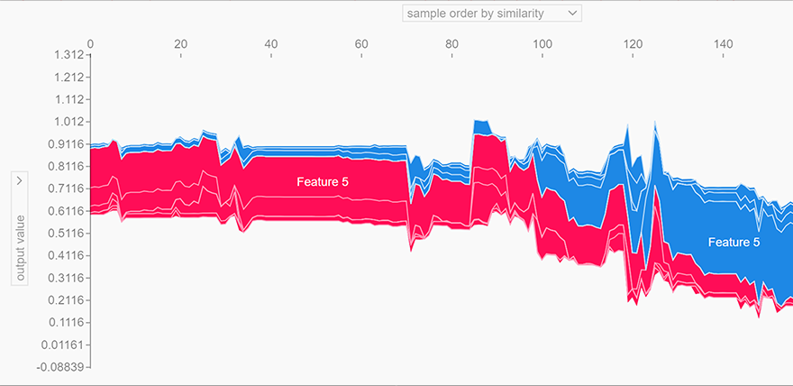
shap.force_plot(explainer.expected_value[0], shap_values[0], X_test)
Using 712 background data samples could cause slower run times. Consider using shap.kmeans(data, K) to summarize the background as K weighted samples.
100%|██████████| 179/179 [00:43<00:00,  4.40it/s]
Out[52]:
Visualization omitted, Javascript library not loaded!
Have you run `initjs()` in this notebook? If this notebook was from another user you must also trust this notebook (File -> Trust notebook). If you are viewing this notebook on github the Javascript has been stripped for security. If you are using JupyterLab this error is because a JupyterLab extension has not yet been written.
In [53]:
# Feature 5 = Sex
# Feature 0 = Class
# Feature 2 = Had siblings
# Feature 1 = age
# Feature 4 = Fare
# Feature 3 = Parent / child
shap.summary_plot(shap_values)
In [54]:
X_train
Out[54]:
array([[   3.    ,   28.5   ,    0.    ,    0.    ,    7.2292,    1.    ],
       [   2.    ,   27.    ,    0.    ,    0.    ,   10.5   ,    0.    ],
       [   3.    ,   25.    ,    1.    ,    0.    ,   16.1   ,    0.    ],
       ..., 
       [   1.    ,   25.    ,    0.    ,    0.    ,  221.7792,    1.    ],
       [   3.    ,   12.    ,    1.    ,    0.    ,   11.2417,    1.    ],
       [   2.    ,   36.    ,    0.    ,    0.    ,   10.5   ,    1.    ]])